Conditional Formatting in Google Sheets (Complete Guide) | Layer Blog (2024)

Conditional formatting is a useful function that allows users to highlight certain cells if they meet specific criteria. There are many ways you can use conditional formatting for your needs, in a variety of situations. You can use the conditional formatting feature in Google Sheets to highlight specific values, format specific cells, and even identify duplicate content. This can make Google Sheets more user-friendly and more intuitive to understand, even for team members who are not familiar with Google Sheets.

One of the very many examples of using conditional formatting is if I have a dataset containing my sales member’s performance data, including their number of clients and total sales. Let’s say I want to highlight the names of all your sales team who have hit their monthly targets. You can do this quite easily, even dynamically as data is updated. Conditional formatting will change the color of cells when certain criteria are met, meaning that you can track progress in a variety of metrics at a glance.

In this article, you’ll learn how conditional formatting works in Google Sheets, knowing exactly how and when to use it. You’ll learn the basics of conditional formatting, how to use custom formulae to create specific conditions for your data, and also how to perform specific actions such as conditional formatting using multiple conditions, conditional formatting based on another cell, and, finally, conditional formatting to find duplicates.

What is conditional formatting?

Conditional formatting allows you to set rules associated with a particular cell(s). When these rules are met or fulfilled, you can specify a change to the visual aspect of the cell itself. These changes usually involve changing the color of a cell, but you can also change the text style within a cell. The conditional formatting feature in Google Sheets is made up of various drop-down menus where you can select your rules and apply it to your data easily.

You can set rules for each cell (or group of cells) using an “if/then” statement made up of the following elements:

For example, let’s say I want to fulfill the following if/then statement: “If cell A1 is not empty then change the cell’s background color to green”. I can use the dropdown menus provided within the conditional formatting feature to create this statement, as you can see in the screenshot below.

How to use conditional formatting in Google Sheets – Range format cells if if/then formatting style

How to use conditional formatting in Google Sheets?

There are many different ways you can use conditional formatting in Google Sheets, depending on your type of data or your desired action.

Let’s take the example mentioned above regarding a sales performance dataset. Using conditional formatting, I can highlight key data values, such as the highest or lowest sales or number of clients, highlight total sales that are within a certain range, or even find duplicate content. First, let’s go through a step-by-step for the most basic way to use the conditional formatting feature in Google Sheets.

There are two options when using conditional formatting in Google Sheets: “Single color”, and “Color scale”. Let’s explore how to use both.

How to use conditional formatting in Google Sheets: Single color

In this example, I want to highlight all of the total sales below $5,000 in red.

1. Open up your Google Sheets file containing your data. Select the cells you want your conditional formatting rule to apply to (eg. ‘D1:D45’) and go to Format > Conditional formatting.

How to use conditional formatting in Google Sheets – Range cursor apply for conditional formatting

2. The menu should appear on the right-hand side of your screen. Make sure you are on the “Single color” tab. As you can see, the cell range has already been set.

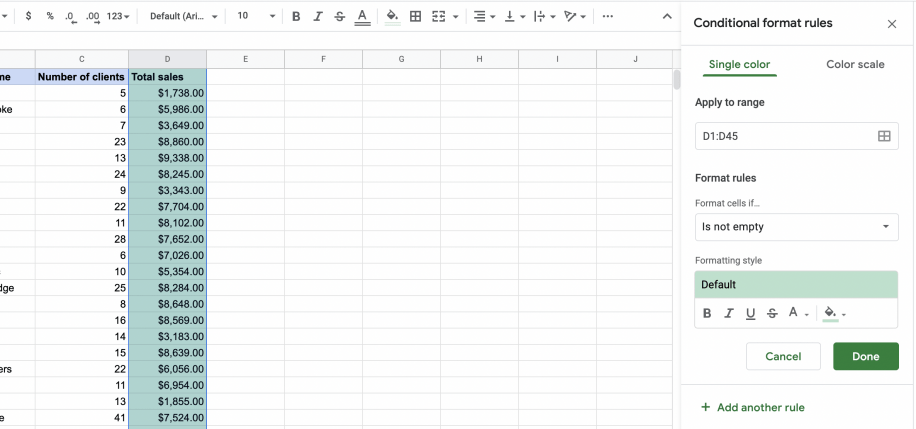
How to use conditional formatting in Google Sheets – Conditional formatting feature Google Sheets

3. Determine the formatting rule. From the dropdown menu under “Format cells if”, choose the condition that you need to trigger the rule. For example, if I want to highlight all of the total sales data below $5,000, I will select the “Less than” option. In the “Value or formula” field below, I will input ‘5,000’.

How to use conditional formatting in Google Sheets – Format cells if

4. Under “Formatting style”, specify the formatting for the cells that fulfill your rule. In this example, let’s set the cell background color to red. Once finished, click “Done”

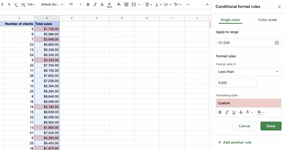
How to use conditional formatting in Google Sheets – Set formatting style

5. Your conditional formatting rules will be applied to your data. As you can see, all of the total sales below $5,000 are now highlighted in red.

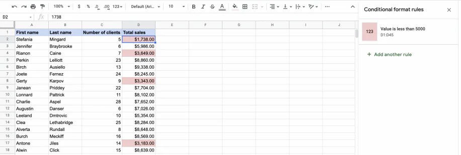
How to use conditional formatting in Google Sheers – Conditional formatting applied to dataset

You can also use the same steps to create formatting conditions greater than cells. Simply change the “Format cells if” drop-down to “Greater than” and add your value.

How to use conditional formatting in Google Sheets: Color scale

Now let’s say I want to apply a color scale to the ‘Total sales’ column. With this option, each cell background will become a different color or shade depending on its value. In this example, I want the lower total sales in red and the higher total sales in green.

1. Just like the previous section, highlight your cell range and open the conditional formatting feature. This time, make sure you have selected the “Color scale” tab.

How to use conditional formatting in Google Sheets – Conditional formatting color scale

2. Under the “Preview” section, click on the color scale and choose the palette your prefer. In order to fulfill my objective, I’ll choose the red-to-green scale.

How to use conditional formatting in Google Sheets – Color scale preview

3. Next, choose the minpoint, midpoint, and maxpoint values and colors. Choose from the dropdown menus of each section the value you wish to base the colors from. To alter the colors, click on the paint can icons and select your preferred color. Once finished, click “Done”

How to use conditional formatting in Google Sheets – set minpoint, midpoint and maxpoint values and colors

4. Your conditional formatting rules will be applied to your data. As you can see, the lowest total sales values are in the red color and the highest values in green.

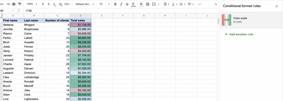
How to use conditional formatting in Google Sheets – Color scale applied to dataset

How to use conditional formatting using a custom formula?

Using a custom formula as part of your conditional formatting is an extremely useful thing indeed. Not only does it give you the opportunity to create more personalized rules that can provide the exact outcome you want, but they can also be used to achieve other important objectives, as you will see further on in this blog post. You can use different functions such as the IF formula for conditional formatting that may help you solve more complex objectives. First, let’s explore how to use the custom formula to create formatting rules.

In this example, I want to highlight all the total sales that are between $4,000-$8,000 in orange. I can add a simple AND formula to achieve this quickly and easily.

How to use conditional formatting in Google Sheets – Custom formula

3. Under “Formatting style”, specify the formatting for the cells that fulfill your rule. In this example, I will set it to orange. Once finished, click “Done”.

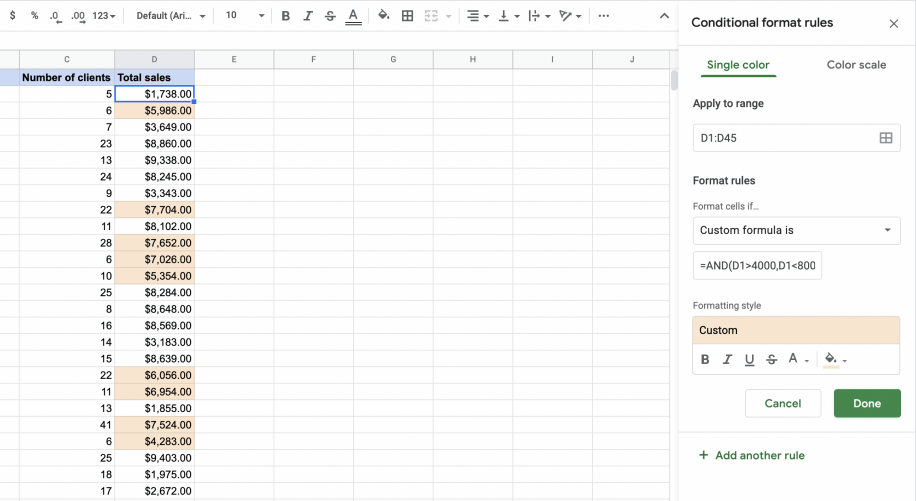
How to use conditional formatting in Google Sheets – Use custom formula as condition

As you can see below, all of the total sales between $4,000 and $8,000 have an orange cell background.

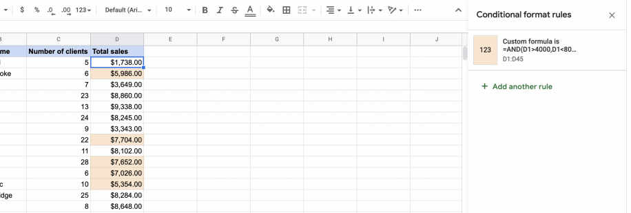
How to use conditional formatting in Google Sheets – Apply custom formula formatting to dataset

How to use conditional formatting based on another cell?

You can also change the color of a cell based on the value of another cell. This may be helpful when dealing with data that rely on each other a lot, or where you have a lot of dynamic data. This is one of the circ*mstances in which you need to use a custom formula. In this example, let’s say I want to highlight the names of the sales team who have less than 10 clients in red. In this example, the formatting of the sales team cells relies on the value of the number of clients.

How to use conditional formatting in Google Sheets – Formatting based on another cell

How to use conditional formatting in Google Sheets – Conditional formatting on another cell

How to use conditional formatting in Google Sheets with multiple conditions?

There may be instances where you want to apply more than one condition to your data. Google Sheets’s conditional formatting feature allows you to create and apply multiple conditions to your data very easily. In this example, let’s say I want to highlight two things; the sales member with the highest total sales, and the one with the lowest total sales. This allows you to compare two columns of data at the same time. For this, we also need to use custom formulae for each rule. First, we need to create the first condition for the maximum sales total. Then we need to create another condition for the minimum sales total.

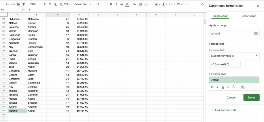
How to use conditional formatting in Google Sheets – Multiple conditions custom formula

3. Now click “+ Add another rule”.

How to use conditional formatting in Google Sheets – Add another rule

4. Create your second rule using the custom formula. In this example, let’s set up the minimum total sales condition using the custom formula =D:D=min(D:D) and changing the color to red. Click “Done”.

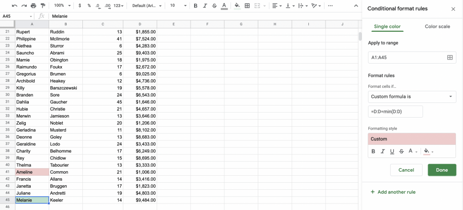
How to use conditional formatting in Google Sheets – Add another condition

5. As you can see, after applying multiple conditions, I now know that Melanie was top in total sales, and Ameline was the bottom.

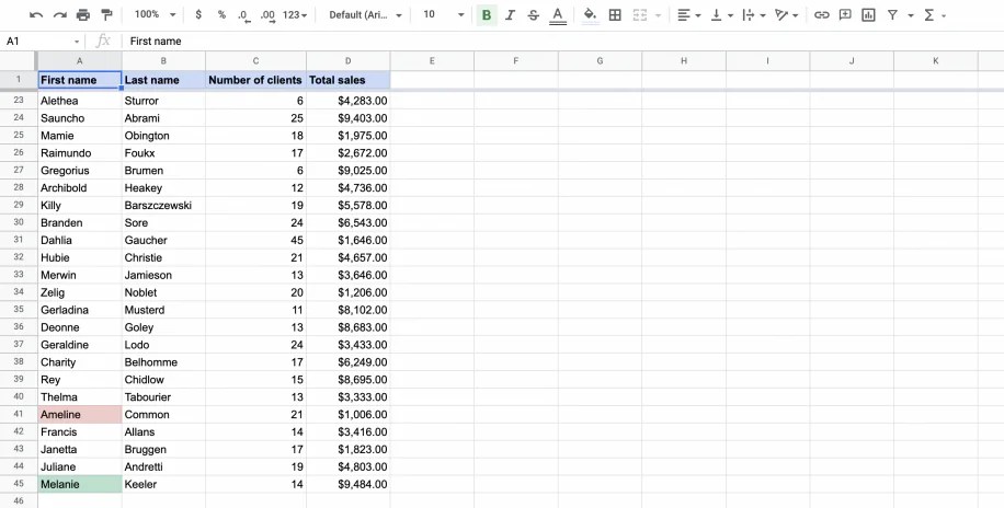
How to use conditional formatting in Google Sheets – Applying multiple conditions to dataset

Conditional formatting to find duplicates

Finally, conditional formatting is very useful for finding duplicate data in your Google Sheets. There are a few ways to do this, depending on where you are looking for duplicates within the data. All of these ways include using a custom formula.

Conditional formatting to find duplicates in a column

Let’s say I want to see whether any of my sales team members’ names have been repeated in my dataset. I can use the COUNTIF formula as my format rule to highlight any duplicates.

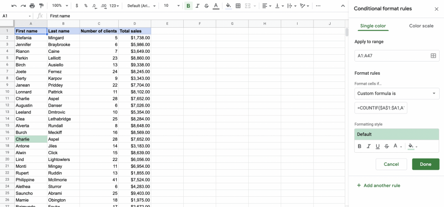
How to use conditional formatting in Google Sheets – Custom formula find duplicates in single column

As you can see from the screenshot above, Charlie’s name has been highlighted as a duplicate.

Conditional formatting to find duplicates in multiple columns

To find duplicates across a range of columns, follow these steps:

3. Apply your “Formatting style” preferences and click “Done”.

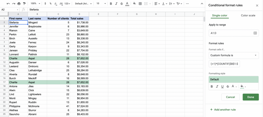
How to use conditional formatting in Google Sheets – Custom formula find duplicates in multiple columns

As you can see from the screenshot above, Each duplicate cell has been highlighted.

Conclusion

Conditional formatting is a powerful and versatile tool that can help you to not only identify specific data but also help you avoid duplicate content. What’s more, conditional formatting in Google Sheets is dynamic – as data is updated, rules will be triggered, so that you always have the most accurate, up-to-date insights.

Now that you have come to the end of this article, you should be able to apply basic conditional formatting to your datasets, use custom formulas to create rules, and find duplicate data effectively. Take a look at our other blog posts for more Google Sheets-related how-to’s.